Guide to Building Probabilistic Models¶

Getting Started with Probabilistic Models¶

InferPy focuses on hirearchical probabilistic models structured in two different layers:

A prior model defining a joint distribution \(p(\mathbf{w})\) over the global parameters of the model. \(\mathbf{w}\) can be a single random variable or a bunch of random variables with any given dependency structure.
A data or observation model defining a joint conditional distribution \(p(\mathbf{x},\mathbf{z}|\mathbf{w})\) over the observed quantities \(\mathbf{x}\) and the the local hidden variables \(\mathbf{z}\) governing the observation \(\mathbf{x}\). This data model is specified in a single-sample basis. There are many models of interest without local hidden variables, in that case, we simply specify the conditional \(p(\mathbf{x}|\mathbf{w})\). Similarly, either \(\mathbf{x}\) or \(\mathbf{z}\) can be a single random variable or a bunch of random variables with any given dependency structure.

For example, a Bayesian PCA model has the following graphical structure,

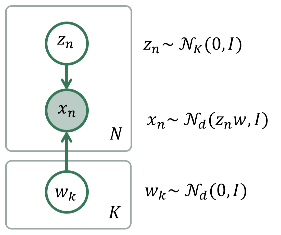
Bayesian PCA

The prior model are the variables \(w_k\). The data model is the part of the model surrounded by the box indexed by N.

And this is how this Bayesian PCA model is denfined in InferPy:

import edward as ed
import inferpy as inf
from inferpy.models import Normal

K, d, N = 5, 10, 200

# model definition
with inf.ProbModel() as m:
    #define the weights
    with inf.replicate(size=K):
        w = Normal(0, 1, dim=d)

    # define the generative model
    with inf.replicate(size=N):
        z = Normal(0, 1, dim=K)
        x = Normal(inf.matmul(z,w), 1.0, observed=True, dim=d)

m.compile()

The with inf.replicate(size = N) sintaxis is used to replicate the random variables contained within this construct. It follows from the so-called plateau notation to define the data generation part of a probabilistic model. Every replicated variable is conditionally idependent given the previous random variables (if any) defined outside the with statement.

Random Variables¶

Following Edward’s approach, a random variable \(x\) is an object parametrized by a tensor \(\theta\) (i.e. a TensorFlow’s tensor or numpy’s ndarray). The number of random variables in one object is determined by the dimensions of its parameters (like in Edward) or by the ‘dim’ argument (inspired by PyMC3 and Keras):

import inferpy as inf
import tensorflow as tf
import numpy as np

# different ways of declaring 1 batch of 5 Normal distributions

x = inf.models.Normal(loc = 0, scale=1, dim=5)         # x.shape = [5]

x = inf.models.Normal(loc = [0, 0, 0, 0, 0], scale=1)  # x.shape = [5]

x = inf.models.Normal(loc = np.zeros(5), scale=1)      # x.shape = [5]

x = inf.models.Normal(loc = 0, scale=tf.ones(5))       # x.shape = [5]

The with inf.replicate(size = N) sintaxis can also be used to define multi-dimensional objects:

with inf.replicate(size=10):
    x = inf.models.Normal(loc=0, scale=1, dim=10)       # x.shape = [10,5]

Following Edward’s approach, the multivariate dimension is the innermost (right-most) dimension of the parameters.

Any random variable in InferPy contain the following (optional) input parameters in the constructor:

validate_args : Python boolean indicating that possibly expensive checks with the input parameters are enabled. By default, it is set to False.
allow_nan_stats : When True, the value “NaN” is used to indicate the result is undefined. Otherwise an exception is raised. Its default value is True.
name: Python string with the name of the underlying Tensor object.
observed: Python boolean which is used to indicate whether a variable is observable or not . The default value is False
dim`: dimension of the variable. The default value is ``None

Inferpy supports a wide range of probability distributions. Details of the specific arguments for each supported distributions are specified in the following sections.

`

Probabilistic Models¶

A probabilistic model defines a joint distribution over observable and non-observable variables, \(p(\mathbf{w}, \mathbf{z}, \mathbf{x})\) for the running example. The variables in the model are the ones defined using the with inf.ProbModel() as pca: construct. Alternatively, we can also use a builder,

m = inf.ProbModel(varlist=[w,z,x])
m.compile()

The model must be compiled before it can be used.

Like any random variable object, a probabilistic model is equipped with methods such as sample(), log_prob() and sum_log_prob(). Then, we can sample data from the model and compute the log-likelihood of a data set:

data = m.sample(1000)
log_like = m.log_prob(data)
sum_log_like = m.sum_log_prob(data)

Random variables can be involved in expressive deterministic operations. Dependecies between variables are modelled by setting a given variable as a parameter of another variable. For example:

with inf.ProbModel() as m:
    theta = inf.models.Beta(0.5,0.5)
    z =  inf.models.Categorical(probs=[theta, 1-theta], name="z")


m.sample()

Moreover, we might consider using the function inferpy.case as the parameter of other random variables:

# Categorical variable depending on another categorical variable

with inf.ProbModel() as m2:
    y =  inf.models.Categorical(probs=[0.4,0.6], name="y")
    x = inf.models.Categorical(probs=inf.case({y.equal(0): [0.0, 1.0],
                                               y.equal(1): [1.0, 0.0] }), name="x")
m2.sample()


# Categorical variable depending on a Normal distributed variable

with inf.ProbModel() as m3:
    a = inf.models.Normal(0,1, name="a")
    b = inf.models.Categorical(probs=inf.case({a>0: [0.0, 1.0],
                                               a<=0: [1.0, 0.0]}), name="b")
m3.sample()


# Normal distributed variable depending on a Categorical variable

with inf.ProbModel() as m4:
    d =  inf.models.Categorical(probs=[0.4,0.6], name="d")
    c = inf.models.Normal(loc=inf.case({d.equal(0): 0.,
                                        d.equal(1): 100.}), scale=1., name="c")
m4.sample()

Supported Probability Distributions¶

Supported probability distributions are located in the package inferpy.models. All of them have inferpy.models.RandomVariable as superclass. A list with all the supported distributions can be obtained as as follows.

>>> inf.models.ALLOWED_VARS
['Bernoulli', 'Beta', 'Categorical', 'Deterministic', 'Dirichlet', 'Exponential', 'Gamma', 'InverseGamma', 'Laplace', 'Multinomial', 'Normal', 'Poisson', 'Uniform']

Bernoulli¶

Binary distribution which takes the value 1 with probability \(p\) and the value with \(1-p\). Its probability mass function is

\[\begin{split}p(x;p) =\left\{\begin{array}{cc} p & \mathrm{if\ } x=1 \\ 1-p & \mathrm{if\ } x=0 \\ \end{array} \right.\end{split}\]

An example of definition in InferPy of a random variable following a Bernoulli distribution is shown below. Note that the input parameter probs corresponds to \(p\) in the previous equation.

x = inf.models.Bernoulli(probs=[0.5])

# or

x = inf.models.Bernoulli(logits=[0])

This distribution can be initialized by indicating the logit function of the probability, i.e., \(logit(p) = log(\frac{p}{1-p})\).

Beta¶

Continuous distribution defined in the interval \([0,1]\) and parametrized by two positive shape parameters, denoted \(\alpha\) and \(\beta\).

\[p(x;\alpha,\beta)=\frac{x^{\alpha-1}(1-x)^{\beta-1}}{B(\alpha,\beta)}\]

where B is the beta function

\[B(\alpha,\beta)=\int_{0}^{1}t^{\alpha-1}(1-t)^{\beta-1}dt\]

The definition of a random variable following a Beta distribution is done as follows.

x = inf.models.Beta(concentration0=0.5, concentration1=0.5)

# or simply:

x = inf.models.Beta(0.5,0.5)

Note that the input parameters concentration0 and concentration1 correspond to the shape parameters \(\alpha\) and \(\beta\) respectively.

Categorical¶

Discrete probability distribution that can take \(k\) possible states or categories. The probability of each state is separately defined:

\[p(x;\mathbf{p}) = p_i\]

where \(\mathbf{p} = (p_1, p_2, \ldots, p_k)\) is a k-dimensional vector with the probability associated to each possible state.

The definition of a random variable following a Categorical distribution is done as follows.

x = inf.models.Categorical(probs=[0.5,0.5])

# or

x = inf.models.Categorical(logits=[0,0])

Deterministic¶

The deterministic distribution is a probability distribution in a space (continuous or discrete) that always takes the same value \(k_0\). Its probability density (or mass) function can be defined as follows.

\[\begin{split}p(x;k_0) =\left\{\begin{array}{cc} 1 & \mathrm{if\ } x=k_0 \\ 0 & \mathrm{if\ } x \neq k_0 \\ \end{array} \right.\end{split}\]

The definition of a random variable following a Beta distribution is done as follows:

x = inf.models.Deterministic(loc=5)

where the input parameter loc corresponds to the value \(k_0\).

Dirichlet¶

Dirichlet distribution is a continuous multivariate probability distribution parmeterized by a vector of positive reals \((\alpha_1,\alpha_2,\ldots,\alpha_k)\). It is a multivariate generalization of the beta distribution. Dirichlet distributions are commonly used as prior distributions in Bayesian statistics. The Dirichlet distribution of order \(k \geq 2\) has the following density function.

\[p(x_1,x_2,\ldots x_k; \alpha_1,\alpha_2,\ldots,\alpha_k) = {\frac{\Gamma\left(\sum_i \alpha_i\right)} {\prod_i \Gamma(\alpha_i)} \prod_{i=1}^k x_i^{\alpha_i-1}}{}\]

The definition of a random variable following a Beta distribution is done as follows:

x = inf.models.Dirichlet(concentration=[5,1])

# or simply:

x = inf.models.Dirichlet([5,1])

where the input parameter concentration is the vector \((\alpha_1,\alpha_2,\ldots,\alpha_k)\).

Exponential¶

The exponential distribution (also known as negative exponential distribution) is defined over a continuous domain and describes the time between events in a Poisson point process, i.e., a process in which events occur continuously and independently at a constant average rate. Its probability density function is

\[\begin{split}p(x;\lambda) =\left\{\begin{array}{cc} \lambda e^{-\lambda x} & \mathrm{if\ } x\geq 0 \\ 0 & \mathrm{if\ } x < k_0 \\ \end{array} \right.\end{split}\]

where \(\lambda>0\) is the rate or inverse scale.

The definition of a random variable following a exponential distribution is done as follows:

x = inf.models.Exponential(rate=1)

# or simply

x = inf.models.Exponential(1)

where the input parameter rate corresponds to the value \(\lambda\).

Gamma¶

The Gamma distribution is a continuous probability distribution parametrized by a concentration (or shape) parameter \(\alpha>0\), and an inverse scale parameter \(\lambda>0\) called rate. Its density function is defined as follows.

\[p(x;\alpha, \beta) = \frac{\beta^\alpha x^{\alpha - 1} e^{\beta x}}{\Gamma(\alpha)}\]

for \(x > 0\) and where \(\Gamma(\alpha)\) is the gamma function.

The definition of a random variable following a gamma distribution is done as follows:

x = inf.models.Gamma(concentration=3, rate=2)

where the input parameters concentration and rate corespond to \(\alpha\) and \(\beta\) respectively.

Inverse-gamma¶

The Inverse-gamma distribution is a continuous probability distribution which is the distribution of the reciprocal of a variable distributed according to the gamma distribution. It is also parametrized by a concentration (or shape) parameter \(\alpha>0\), and an inverse scale parameter \(\lambda>0\) called rate. Its density function is defined as follows.

\[p(x;\alpha, \beta) = \frac{\beta^\alpha x^{-\alpha - 1} e^{-\frac{\beta}{x}}}{\Gamma(\alpha)}\]

for \(x > 0\) and where \(\Gamma(\alpha)\) is the gamma function.

The definition of a random variable following a inverse-gamma distribution is done as follows:

x = inf.models.InverseGamma(concentration=3, rate=2)

where the input parameters concentration and rate corespond to \(\alpha\) and \(\beta\) respectively.

Laplace¶

The Laplace distribution is a continuous probability distribution with the following density function

\[p(x;\mu,\sigma) = \frac{1}{2\sigma} exp \left( - \frac{|x - \mu |}{\sigma}\right)\]

The definition of a random variable following a Beta distribution is done as follows:

x = inf.models.Laplace(loc=0, scale=1)

# or simply

x = inf.models.Laplace(0,1)

where the input parameter loc and scale correspond to \(\mu\) and \(\sigma\) respectively.

Multinomial¶

The multinomial is a discrete distribution which models the probability of counts resulting from repeating \(n\) times an experiment with \(k\) possible outcomes. Its probability mass function is defined below.

\[p(x_1,x_2,\ldots x_k; \mathbf{p}) = \frac{n!}{\prod_{i=1}^k x_i}\prod_{i=1}^k p_i^{x^i}\]

where \(\mathbf{p}\) is a k-dimensional vector defined as \(\mathbf{p} = (p_1, p_2, \ldots, p_k)\) with the probability associated to each possible outcome.

The definition of a random variable following a multinomial distribution is done as follows:

x = inf.models.Multinomial(total_count=4, probs=[0.5,0.5])

# or

x = inf.models.Multinomial(total_count=4, logits=[0,0])

Normal¶

The normal (or Gaussian) distribution is a continuous probability distribution with the following density function

\[p(x;\mu,\sigma) = \frac{1}{2\sigma} exp \left( - \frac{|x - \mu |}{\sigma}\right)\]

where \(\mu\) is the mean or expectation of the distribution, \(\sigma\) is the standard deviation, and \(\sigma^{2}\) is the variance.

A normal distribution can be defined as follows.

x = inf.models.Normal(loc=0, scale=1)

# or

x = inf.models.Normal(0,1)

where the input parameter loc and scale correspond to \(\mu\) and \(\sigma\) respectively.

Poisson¶

The Poisson distribution is a discrete probability distribution for modelling the number of times an event occurs in an interval of time or space. Its probability mass function is

\[p(x;\lambda) = e^{- \lambda} \frac{\lambda^x}{x!}\]

where \(\lambda\) is the rate or number of events per interval.

A Poisson distribution can be defined as follows.

x = inf.models.Poisson(rate=4)

# or

x = inf.models.Poisson(4)

Uniform¶

The continuous uniform distribution or rectangular distribution assings the same probability to any \(x\) in the interval \([a,b]\).

\[\begin{split}p(x;a,b) =\left\{\begin{array}{cc} \frac{1}{b-a} & \mathrm{if\ } x\in [a,b]\\ 0 & \mathrm{if\ } x\not\in [a,b] \\ \end{array} \right.\end{split}\]

A uniform distribution can be defined as follows.

x = inf.models.Uniform(low=1, high=3)

# or

inf.models.Uniform(1,3)

where the input parameters low and high correspond to the lower and upper bounds of the interval \([a,b]\).