Guide to Building Probabilistic Models

Getting Started with Probabilistic Models

InferPy focuses on hirearchical probabilistic models which usually are structured in two different layers:

• A prior model defining a joint distribution \(p(\theta)\) over the global parameters of the model, \(\theta\).
• A data or observation model defining a joint conditional distribution \(p(x,h|\theta)\) over the observed quantities \(x\) and the the local hidden variables \(h\) governing the observation \(x\). This data model should be specified in a single-sample basis. There are many models of interest without local hidden variables, in that case we simply specify the conditional \(p(x|\theta)\). More flexible ways of defining the data model can be found in ?.

A Bayesian PCA model has the following graphical structure,

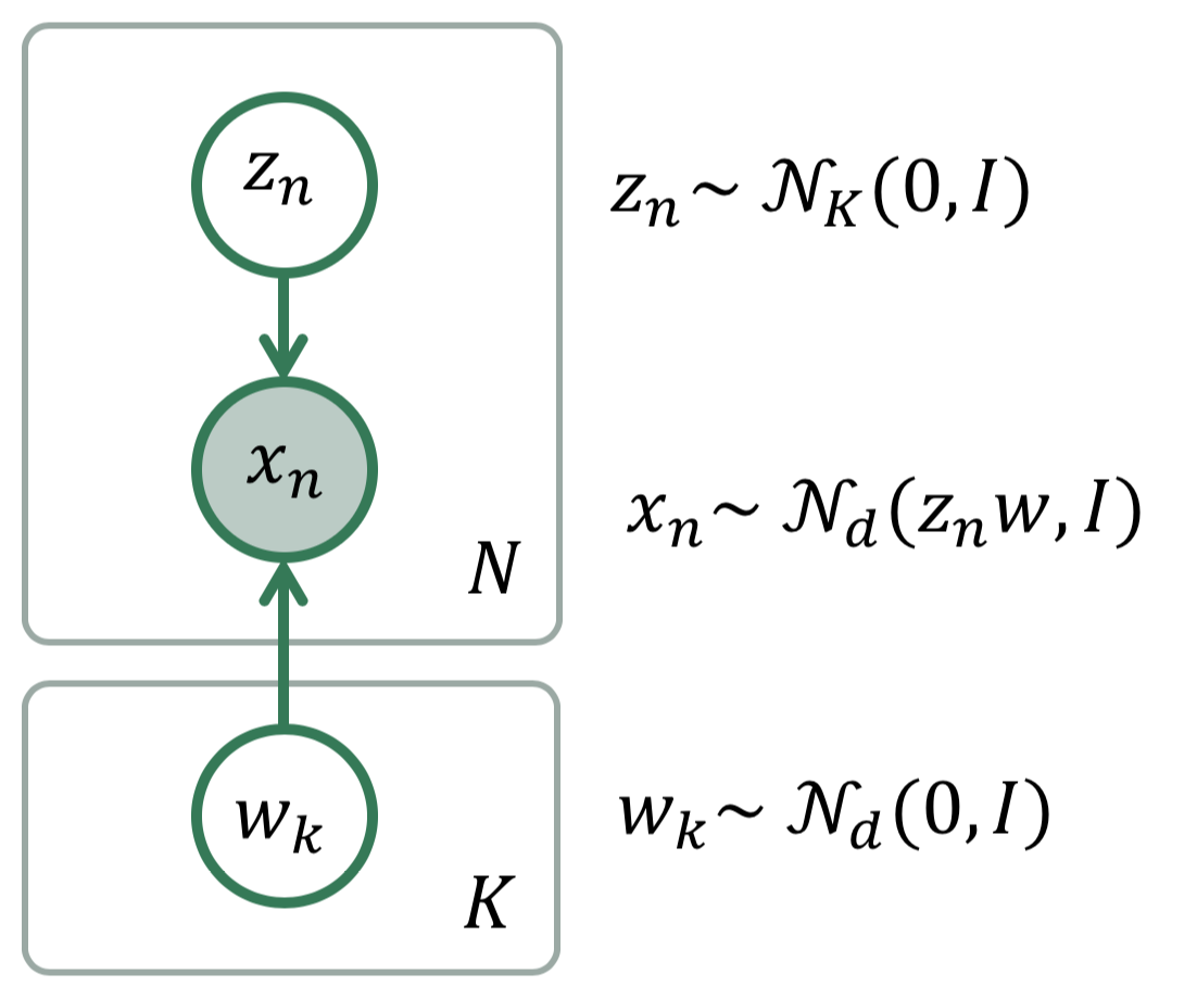
Bayesian PCA

The prior model is the variable \(\mu\). The data model is the part of the model surrounded by the box indexed by N.

And this is how this Bayesian PCA model is denfined in InferPy:

import edward as ed
import inferpy as inf
from inferpy.models import Normal

K, d, N = 5, 10, 200

# model definition
with inf.ProbModel() as m:
    #define the weights
    with inf.replicate(size=K):
        w = Normal(0, 1, dim=d)

    # define the generative model
    with inf.replicate(size=N):
        z = Normal(0, 1, dim=K)
        x = Normal(inf.matmul(z,w), 1.0, observed=True, dim=d)

m.compile()

The with inf.replicate(size = N) sintaxis is used to replicate the random variables contained within this construct. It follows from the so-called plateau notation to define the data generation part of a probabilistic model. Every replicated variable is conditionally idependent given the previous random variables (if any) defined outside the with statement.

Random Variables

Following Edward’s approach, a random variable \(x\) is an object parametrized by a tensor \(\theta\) (i.e. a TensorFlow’s tensor or numpy’s ndarray). The number of random variables in one object is determined by the dimensions of its parameters (like in Edward) or by the ‘dim’ argument (inspired by PyMC3 and Keras):

import inferpy as inf
import tensorflow as tf
import numpy as np


# different ways of declaring 1 batch of 5 Normal distributions

x = inf.models.Normal(loc = 0, scale=1, dim=5)         # x.shape = [5]

x = inf.models.Normal(loc = [0, 0, 0, 0, 0], scale=1)  # x.shape = [5]

x = inf.models.Normal(loc = np.zeros(5), scale=1)      # x.shape = [5]

x = inf.models.Normal(loc = 0, scale=tf.ones(5))       # x.shape = [5]

The with inf.replicate(size = N) sintaxis can also be used to define multi-dimensional objects:

with inf.replicate(size=10):
    x = inf.models.Normal(loc=0, scale=1, dim=10)       # x.shape = [10,5]

Following Edward’s approach, the multivariate dimension is the innermost (right-most) dimension of the parameters.

The argument observed = true in the constructor of a random variable is used to indicate whether a variable is observable or not.

Probabilistic Models

A probabilistic model defines a joint distribution over observable and non-observable variables, \(p(\theta,\mu,\sigma,z_n, x_n)\) for the running example. The variables in the model are the ones defined using the with inf.ProbModel() as pca: construct. Alternatively, we can also use a builder,

m = inf.ProbModel(varlist=[w,z,x])
m.compile()

The model must be compiled before it can be used.

Like any random variable object, a probabilistic model is equipped with methods such as sample(), log_prob() and sum_log_prob(). Then, we can sample data from the model and compute the log-likelihood of a data set:

data = m.sample(1000)
log_like = m.log_prob(data)
sum_log_like = m.sum_log_prob(data)

Folowing Edward’s approach, a random variable \(x\) is associated to a tensor \(x^*\) in the computational graph handled by TensorFlow, where the computations takes place. This tensor \(x^*\) contains the samples of the random variable \(x\), i.e. \(x^*\sim p(x|\theta)\). In this way, random variables can be involved in expressive deterministic operations.

Dependecies between variables are modelled by setting a given variable as a parameter of another variable. For example:

with inf.ProbModel() as m:
    theta = inf.models.Beta(0.5,0.5)
    z =  inf.models.Categorical(probs=[theta, 1-theta], name="z")


m.sample()

Moreover, we might consider using the function inferpy.case as the parameter of other random variables:

# Categorical variable depending on another categorical variable

with inf.ProbModel() as m2:
    y =  inf.models.Categorical(probs=[0.4,0.6], name="y")
    x = inf.models.Categorical(probs=inf.case({y.equal(0): [0.0, 1.0],
                                               y.equal(1): [1.0, 0.0] }), name="x")
m2.sample()


# Categorical variable depending on a Normal distributed variable

with inf.ProbModel() as m3:
    a = inf.models.Normal(0,1, name="a")
    b = inf.models.Categorical(probs=inf.case({a>0: [0.0, 1.0],
                                               a<=0: [1.0, 0.0]}), name="b")
m3.sample()


# Normal distributed variable depending on a Categorical variable

with inf.ProbModel() as m4:
    d =  inf.models.Categorical(probs=[0.4,0.6], name="d")
    c = inf.models.Normal(loc=inf.case({d.equal(0): 0.,
                                        d.equal(1): 100.}), scale=1., name="c")
m4.sample()

Supported Probability Distributions

Supported probability distributions are located in the package inferpy.models. All of them have inferpy.models.RandomVariable as superclass. Those currently implemented are:

>>> inf.models.ALLOWED_VARS
['Bernoulli', 'Beta', 'Categorical', 'Deterministic', 'Dirichlet', 'Exponential', 'Gamma', 'InverseGamma', 'Laplace', 'Multinomial', 'Normal', 'Poisson', 'Uniform']