Getting Started: 30 seconds to InferPy
The core data structures of InferPy is a probabilistic model, defined as a set of random variables with a conditional independence structure. Like in Edward, a random varible is an object parameterized by a set of tensors.
Let’s look at a simple (Bayesian) probabilistic component analysis model. Graphically the model can be defined as follows,
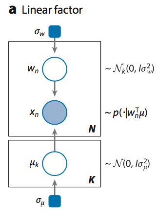
Bayesian PCA
We start defining the prior of the global parameters,
import numpy as np
import inferpy as inf
from inferpy.models import Normal, InverseGamma, Dirichlet

# K defines the number of components.
K=10

# d defines the number of dimensions
d=20

#Prior for the principal components
with inf.replicate(size = K)
    mu = Normal(loc = 0, scale = 1, dim = d)
InferPy supports the definition of plateau notation by using the
construct with inf.replicate(size = K), which replicates K times the
random variables enclosed within this anotator. Every replicated
variable is assumed to be independent.
This with inf.replicate(size = N) construct is also useful when
defining the model for the data:
# Number of observations
N = 1000

#data Model
with inf.replicate(size = N):
    # Latent representation of the sample
    w_n = Normal(loc = 0, scale = 1, dim = K)
    # Observed sample. The dimensionality of mu is [K,d].
    x = Normal(loc = mu0 + inf.matmul(w_n,mu), scale = 1.0, observed = true)
As commented above, the variable w_n and x_n are surrounded by a
with statement to inidicate that the defined random variables will
be reapeatedly used in each data sample. In this case, every replicated
variable is conditionally idependent given the variables mu and sigma
defined outside the with statement.
Once the random variables of the model are defined, the probablitic model itself can be created and compiled. The probabilistic model defines a joint probability distribuiton over all these random variables.
from inferpy import ProbModel

# Define the model
pca = ProbModel(vars = [mu,w_n,x_n])

# Compile the model
pca.compile(infMethod = 'KLqp')
During the model compilation we specify different inference methods that will be used to learn the model.
from inferpy import ProbModel

# Define the model
pca = ProbModel(vars = [mu,w_n,x_n])

# Compile the model
pca.compile(infMethod = 'MCMC')
The inference method can be further configure. But, as in Keras, a core principle is to try make things reasonbly simple, while allowing the user the full control if needed.
from keras.optimizers import SGD

# Define the model
pca = ProbModel(vars = [mu,w_n,x_n])

# Define the optimiser
sgd = SGD(lr=0.01, decay=1e-6, momentum=0.9, nesterov=True)

# Define the inference method
infklqp = inf.inference.KLqp(optimizer = sgd, loss="ELBO")

# Compile the model
pca.compile(infMethod = infklqp)
Every random variable object is equipped with methods such as
log_prob() and sample(). Similarly, a probabilistic model is also
equipped with the same methods. Then, we can sample data from the model
anbd compute the log-likelihood of a data set:
# Sample data from the model
data = pca.sample(size = 100)

# Compute the log-likelihood of a data set
log_like = probmodel.log_prob(data)
Of course, you can fit your model with a given data set:
# Fit the model with the given data
pca.fit(data_training, epochs=10)
Update your probablistic model with new data using the Bayes’ rule:
# Update the model with the new data
pca.update(new_data)
Query the posterior over a given random varible:
# Compute the posterior of a given random variable
mu_post = pca.posterior(mu)
Evaluate your model according to a given metric:
# Evaluate the model on given test data set using some metric
log_like = pca.evaluate(test_data, metrics = ['log_likelihood'])
Or compute predicitons on new data
# Make predictions over a target var
latent_representation = pca.predict(test_data, targetvar = w_n)