Guide to Building Probabilistic Models
Getting Started with Probabilistic Models
InferPy focuses on hirearchical probabilistic models which usually are structured in two different layers:
- A prior model defining a joint distribution \(p(\theta)\) over the global parameters of the model, \(\theta\).
- A data or observation model defining a joint conditional distribution \(p(x,h|\theta)\) over the observed quantities \(x\) and the the local hidden variables \(h\) governing the observation \(x\). This data model should be specified in a single-sample basis. There are many models of interest without local hidden variables, in that case we simply specify the conditional \(p(x|\theta)\). More flexible ways of defining the data model can be found in ?.
A Bayesian PCA model has the following graphical structure,
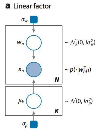
Bayesian PCA
The prior model is the variable \(\mu\). The data model is the part of the model surrounded by the box indexed by N.
And this is how this Bayesian PCA model is denfined in InferPy:
import numpy as np
import inferpy as inf
from inferpy.models import Normal, InverseGamma, Dirichlet

import numpy as np
import inferpy as inf
from inferpy.models import Normal, InverseGamma, Dirichlet

# Define the probabilistic model
with inf.ProbModel() as pca:
   # K defines the number of components.
   K=10

   #Prior for the principal components
   with inf.replicate(size = K)
      mu = Normal(loc = 0, scale = 1, dime = d)

   # Number of observations
   N = 1000

   #data Model
   with inf.replicate(size = N):
      # Latent representation of the sample
      w_n = Normal(loc = 0, scale = 1, dim = K)
      # Observed sample. The dimensionality of mu is [K,d].
      x = Normal(loc = inf.matmul(w_n,mu), scale = 1.0, observed = true)

   #compile the probabilistic model
   pca.compile()
The with inf.replicate(size = N) sintaxis is used to replicate the
random variables contained within this construct. It follows from the
so-called plateau notation to define the data generation part of a
probabilistic model. Every replicated variable is conditionally
idependent given the previous random variables (if any) defined
outside the with statement.
Random Variables
Following Edward’s approach, a random variable \(x\) is an object parametrized by a tensor \(\theta\) (i.e. a TensorFlow’s tensor or numpy’s ndarray). The number of random variables in one object is determined by the dimensions of its parameters (like in Edward) or by the ‘shape’ or ‘dim’ argument (inspired by PyMC3 and Keras):
# matrix of [1, 5] univariate standard normals
x  = Normal(loc = 0, scale = 1, dim = 5)

# matrix of [1, 5] univariate standard normals
x  = Normal(loc = np.zeros(5), scale = np.ones(5))

# matrix of [1,5] univariate standard normals
x = Normal (loc = 0, scale = 1, shape = [1,5])
The with inf.replicate(size = N) sintaxis can also be used to define
multi-dimensional objects:
# matrix of [10,5] univariate standard normals
with inf.replicate(size = 10)
    x = Normal (loc = 0, scale = 1, dim = 5)
Multivariate distributions can be defined similarly. Following Edward’s approach, the multivariate dimension is the innermost (right-most) dimension of the parameters.
# Object with five K-dimensional multivariate normals, shape(x) = [5,K]
x  = MultivariateNormal(loc = np.zeros([5,K]), scale = np.ones([5,K,K]))

# Object with five K-dimensional multivariate normals, shape(x) = [5,K]
x = MultivariateNormal (loc = np.zeros(K), scale = np.ones([K,K]), shape = [5,K])
The argument observed = true in the constructor of a random variable
is used to indicate whether a variable is observable or not.
Probabilistic Models
A probabilistic model defines a joint distribution over observable
and non-observable variables, \(p(\theta,\mu,\sigma,z_n, x_n)\) for the
running example. The variables in the model are the ones defined using the
with inf.ProbModel() as pca: construct. Alternatively, we can also use a builder,
from inferpy import ProbModel
pca = ProbModel(vars = [mu,w_n,x_n])
pca.compile()
The model must be compiled before it can be used.
Like any random variable object, a probabilistic model is equipped with
methods such as log_prob() and sample(). Then, we can sample data
from the model and compute the log-likelihood of a data set:
data = probmodel.sample(size = 1000)
log_like = probmodel.log_prob(data)
Folowing Edward’s approach, a random variable \(x\) is associated to a tensor \(x^*\) in the computational graph handled by TensorFlow, where the computations takes place. This tensor \(x^*\) contains the samples of the random variable \(x\), i.e. \(x^*\sim p(x|\theta)\). In this way, random variables can be involved in expressive deterministic operations. For example, the following piece of code corresponds to a zero inflated linear regression model
#Prior
w = Normal(0, 1, dim=d)
w0 = Normal(0, 1)
p = Beta(1,1)

#Likelihood model
with inf.replicate(size = 1000):
    x = Normal(0,1000, dim=d, observed = true)
    h = Binomial(p)
    y0 = Normal(w0 + inf.matmul(x,w, transpose_b = true), 1),
    y1 = Delta(0.0)
    y = Deterministic(h*y0 + (1-h)*y1, observed = true)

probmodel = ProbModel(vars = [w,w0,p,x,h,y0,y1,y])
probmodel.compile()
data = probmodel.sample(size = 1000)
probmodel.fit(data)
A special case, it is the inclusion of deep neural networks within our probabilistic model to capture complex non-linear dependencies between the random variables. This is extensively treated in the the Guide to Bayesian Deep Learning.
Finally, a probablistic model have the following methods:
probmodel.summary(): prints a summary representation of the model.probmodel.get_config(): returns a dictionary containing the configuration of the model. The model can be reinstantiated from its config via:
config = probmodel.get_config()
probmodel = ProbModel.from_config(config)
model.to_json(): returns a representation of the model as a JSON string. Note that the representation does not include the weights, only the architecture. You can reinstantiate the same model (with reinitialized weights) from the JSON string via: ```python from models import model_from_json
json_string = model.to_json()
model = model_from_json(json_string)